Athelas
A parallel random graph generation library.
                              By
               Karandeep Johar & Eshan Verma
         kjohar@andrew.cmu.edu   everma@andrew.cmu.edu
SUMMARY:
We implemented a library to generate parallel large-scale graphs using OpenMP/pThreads, exploiting CPU Architecture and using CUDA on GPUS. The aim was to compare implementation complexity, speed and resource efficiency.
BACKGROUND:
Processing Real World graphs is an active research problem. The real-world complex graphs are typically very large (with millions or more vertices) and their sizes grow over time. Some researchers predict that the size of these graphs will eventually reach 10^15 vertices. Unfortunately, we do not have publicly available real graphs that are large enough to test the functionality and true scalability of the graph applications. Hence, graph generation is an important field of research. There are many implementation and algorithms that exist but a serious drawback of these models is that they are all sequential models and thus, are inadequate in their usage to generate massive graphs with billions of vertices and edges.
- Stochastic Kronecker Graph (A generalization of RMAT graph generation and ER)
- Erdos-Renyi graph
- Parallel Barabasi-Albert (PBA) method
- CL method (Chung Lu)
To concentrate best on our aim of comparison of the implementation libraries, we implemented the RMAT algorithm which is a generalization on the ER algorithm. The idea was to best optimize this algorithm over the various libraries to analyze the implementation and speedup.
We used SNAP and PaRMAT libraries for initial benchmarking and as code base. The evaluation of our algorithms and benchmarking was implemented by us. The checker functions to ensure that the properties for RMATs were ported from SNAP. Both these libraries provide different options for generations of graphs (directed vs. undirected, sorted vs. unsorted), we modeled our interface to support the same. To get optimal performance, we tuned our kernels/functions to take such parameters in to account.
THE CHALLENGE AND THE TACKLE
Our project is different from most other tasks handled in this course. There is no reading of input data, rather a large amount of data is generated. Since each node is operated on independently, there is a large communication overhead to ensure connectivity amongst the nodes. Also, there is an inherent workload imbalance, the implementation had to be tuned to that particular use-cases. Along with that we ensured the following:
- Reducing communication between different parallel elements
- Distributing graph over the cores (load balancing)
- Writing efficiently to memory
- Compressed representation of the graph
The load-balancing issue is showcased in the graph below. This is the initial cut implementations of our algorithms with skew on the probability distribution mapped on the x-axis.

Workload Distribution of implementation across probabilities
Inputs and Outputs
-Inputs: Probability Distribution (Explained ahead), No. of Edges, No. of Vertices, Graph Properties
-Outputs: Traditionally, a tab separated list of edges (There is a giant inefficiency here which we address later)
-Outputs: Graph in Memory
Unit of Parallelism and Sharding of Squares
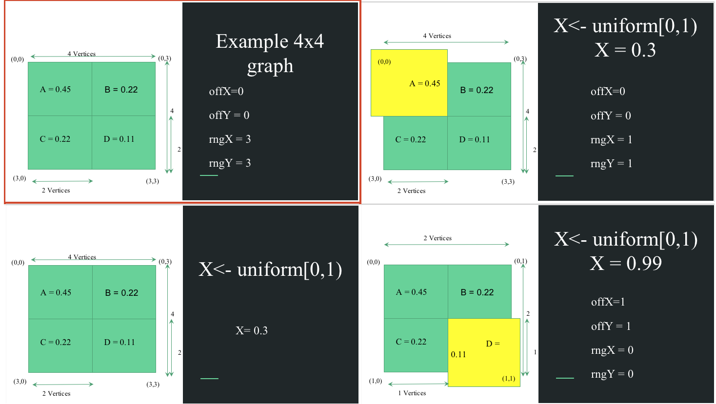
Generation of edge (1,1) in a 4x4 Matrix
As the Figure above shows, a computation of an edge requires calculation of random uniform probabilities and recursively looking up the probability distribution of the graph to be generated. Hence, implicitly, a parallelism exists over every edge. However, it is wiser to shard over sub-squares, or sub-quadrants. The reason being, the communication and synchronization overhead over all edges will be more than determining a distribution of the number of edges within a square and hence parallelizing over these modules. Thus each square will call recursively try to generate its share of edges till its pool of edges to generate is exhausted. This ensures that the net edges to generate is preserved. Another factor which is benefitted from this approach is load balancing as we can ensure work distribution amongst sub-squares.
APPROACH
There are three parts in the approach we adopted: (1) A Serial CPU Square Generation: All three implementations share a serial section in which the input matrix of edges to be generated is divided up in squares according to the probability distributions and these squares get a connection degree associated with them. As explained before, this has some inherent advantages. The division can be seen in the figure.
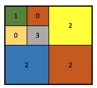
Square Generation across which parallelism is maintained
NOTE: In our analysis, we have excluded timing of this section as a fixed overhead.
The next part was implemented differently according to the various optimizations available in the three libraries.
(2.a) PTHREADs based Graph Generation: We followed a worker-queue based implementation for both scheduling the generation of the graph and writing it to file. The optimization over the baseline was better load balancing by scheduling squares better and determining size of squares better. The latency of writing to files was hidden by following a producer-consumer queue and the master thread handling all writes.
(2.b) openMP Graph Generation: The openMP implementation was over all the squares in the list, and having a lock over over writing to file. The motivation behind this was to avoid having one thread idle during generation and have threads scheduled out while waiting over the lock so that generation time could be reduced.
(2.c) CUDA Graph Generation: The kernel design for CUDA involved optimizing over sorted vs. non-sorted graph. At the block level we parallelized over all squares and within a block, the parallellization was over all source nodes. The graph was compressed by writing matrix offsets of edges generated to memory. Hence the compression of the graph helped in reducing the memory transfer overhead from the device. At the same time, the cost of expanding the graph is not much in the CPU. The serial algorithm for sorting was optimized to gain block locality and benefit from shared memory accesses as opposed to flushing to global memory. Another overhead in CUDA was ensuring the random number generation for which we had to initialize different states for graph depth and thread ID. The CURAND library was used for generating a random number from within the kernel.
Paths not Taken
We tried implementing the Poisson-SKG algorithm which enables one to generate a set of destination edges from one source in a single iteration. However, the output graphs were very noisy, and even though this implementation had benefits we abandoned it as the noisy graphs did not align with our correctness measure.
RESULTS
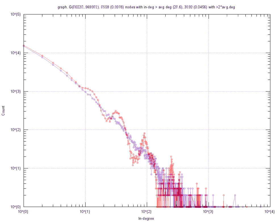
Error correction in original code
We can see that the original implementation(in red) had a bug and did not actually get the in-degree curve that we were looking for in a RMAT graph(our implementation in purple). This was an algorithmic change that was needed to ensure correctness as reported by SNAP. The same is ensured across implementations.
NOTE: Aside on Timing information:
- OpenMP and PTHREADs have only the graph generation time mentioned with FILE IO being kept separate. We are in the process of optimizing FILE IO for these and the times will be updated over the weekend.
- CUDA runtimes includes time for generation and the data transfer time HtoD. As above FILE IO is in the process of being optimized through parallel stream execution and will be updated over the weekend.
- All profiling done was using CycleTimer in CPU and NVPROF on GPU. Graph being generated is with 100k vertices and 1 million edges unless stated otherwise.
- The comparisons are pre-compression. Comparison data is presented for CUDA in the last section.
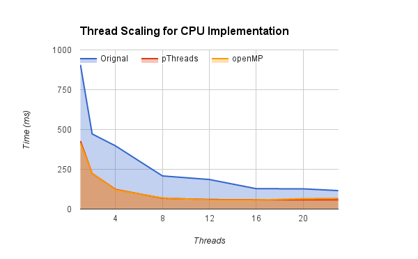
Scaling of code across nCores of CPU
Our implementation scales across cores and plateaus after a point as the inherent parallelism breaks down.
We are not comparing generation speedup w.r.t. the baseline input as there were some logical faults in the graph generation algorithm, however, we can compare our algorithm across the 3 libraries as its uniform and correct. As can be seen PTHREADs is having an advantage over openMP due to the better distribution and no overheads. CUDA, even with the device transfer is performing an order faster than both.
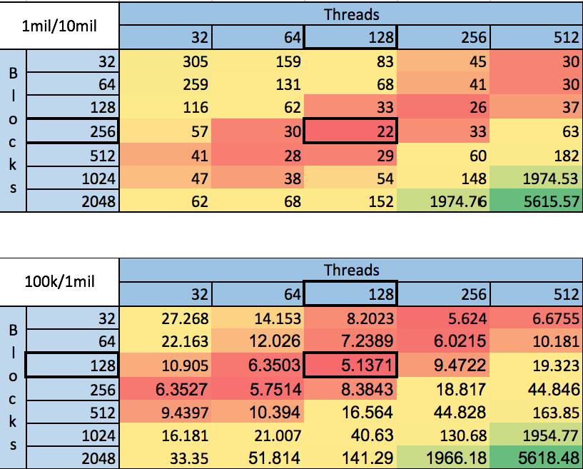
CUDA Tuning Challenges on scaling generated vertices 10x and edges 10x
One inherent challenge in CUDA is finding the sweet spot of implementation in terms of thread and block sizing. This is visualized above with scaling the vertices and edges by 10x. As can be seen the sweet spot shifts. We could heuristically tune this parameter based on sparsity of the target matrix but such an approach was not adopted.
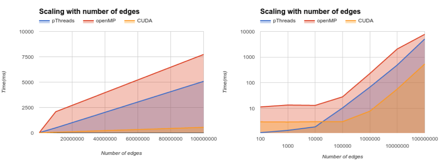
Overall scaling. (L) Linear Time Vs. Linear Scale, (R) Log Time Vs. Log Scale
The overall scaling of all implementations is shown above and as expected, the CUDA generation plus memory times seem to perform much better across scales. However, the Log scale graph showcases that there is a fixed overhead in CUDA for smaller graphs.
Compression
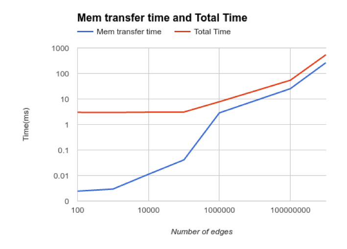 After looking at the memory transfer times we realized that memory copy times are taking a significant amount of time on the GPU. We first looked at the squares and saw that most ranges were less than 2^16. This meant that we can actually fit in the the edge exactly in a 2^32 bit representations of uints.
The idea here was to build a compact representation of the graph so as to minimize the data transfer between device and host. By storing edges in a compact form, we were able to reduce the memory transfer by a factor of 2x on average which is a significant saving. This representation has minimal overhead in the kernel or in terms of reconstruction on the CPU. The basic representation is by storing an edge tuple as a single number instead of a tuple. Within a square each edge can be represented as an offset form the origin, the details of this representation are listed in the Algorithm description below.
After looking at the memory transfer times we realized that memory copy times are taking a significant amount of time on the GPU. We first looked at the squares and saw that most ranges were less than 2^16. This meant that we can actually fit in the the edge exactly in a 2^32 bit representations of uints.
The idea here was to build a compact representation of the graph so as to minimize the data transfer between device and host. By storing edges in a compact form, we were able to reduce the memory transfer by a factor of 2x on average which is a significant saving. This representation has minimal overhead in the kernel or in terms of reconstruction on the CPU. The basic representation is by storing an edge tuple as a single number instead of a tuple. Within a square each edge can be represented as an offset form the origin, the details of this representation are listed in the Algorithm description below.
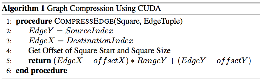
Algorithm for Compression
This also allows for easy reconstruction, as the math pre edge is independent and simple. Thus instead of storing an edge as a tuple, we are storing it as a single integer.
Huffman coding
We looked at the results of this optimization and found that as we increase the number of vertices the number of times that we can actually apply this approach goes down. This is because the range of the square quickly exceeds 2^16 vertices. We then looked at another method for achieving compression.
Unfortunately most other compression formats are ill suited for compressing the graph on the fly as we are generating it. So formats like CSR which are are commonly used in numpy are ill suited for the job.
The key insight is that all edges are not equally likely and hence our level of our surprise should be different for different edges. It should be lower for edges with higher probabilities and higher for ones with lower probabilities. Huffman coding actually formalizes this concept.
We can think of an edge (V1, V2) as a series of choices. At each stage we choose one of the 4 blocks. A,B,C or D. So we can actually represent the edge as [A|B|C|D]+ of length log(|V|). Now, because we know the prior probabilities of a,b,c and d we can encode this string using huffman codes for the the respective blocks.
Say A has a probability mass of 0.9. That would mean that most of the edges would lie in the upper left corner of the graph. This would mean that most edges have a large percentage of As in them. This would give us a huge reason for compression.
Compression Results
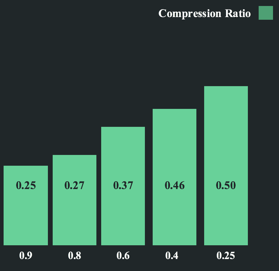
Compression across probabilities
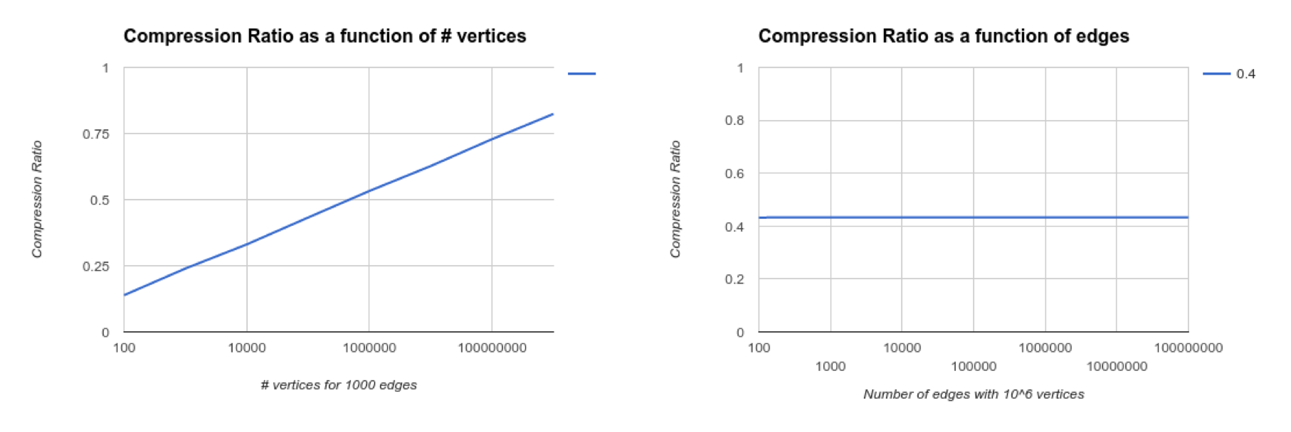
Unsurprisingly the compression ratio for graphs is higher for the cases where the probabilities are really skewed or the number of vertices is smaller than 2^32. The second condition follows from the fact that greater the number of vertices the greater the depth we need to go to actually get the graph. This implies a greater edge string length in terms of blocks for those graphs and lesser scope for compression.
As we increase the number of edges the compression ratio remains constant. This is because the compression ratio per edge is independent of the number of edges.
ASIDE:
A note on programming complexity
Start-to-Basic Implementation OpenMP was the easiest to parallelize a given serial implementation, with PTHREADs involving some restructuring to enable threading and queueing. CUDA was complex to get going due to kernel design overheads, figuring the data transfer and parameter(s) access across devices, as well as random number generation on the GPU.
Optimization Freedom Due to its nature, openMP provided the least options to explore and least flexibility in terms of implementation. CUDA on the other hand is something we are still optimizing over. The chance to exploit block level locality presents many diverse implementation strategies and options.
FUTURE WORK
We want to explore latency hiding in all three for faster memory operations. The use of compression was already implemented in CUDA and needs to be done in the other two. CUDA also has parallel stream execution by which we can transfer chunks of memory the moment a kernel gets over. We will try to finish the experiments by 5/9.
Tl;Dr
We implemented a Parallel Graph Generation Library which enables a user to generate massive random graphs using the platform of choice. The implementation across libraries was to best understand the complexity as well as optimization capabilities of each and not just to present as an option to the end user. The library scales across graph sizes and is easy and intuitive to setup and use.
RESOURCES
- We will be using the code present here as our starting point: "GitHub - ParMAT"
- The details of which are present in this paper: Chakrabarti, Deepayan, Yiping Zhan, and Christos Faloutsos. "R-MAT: A Recursive Model for Graph Mining." SDM. Vol. 4. 2004. Khorasani, Farzad, Rajiv Gupta, and Laxmi N. Bhuyan. "Scalable SIMD-Efficient Graph Processing on GPUs. and
- SNAP, a library out of STANFORD which is based on OpenMPI and we will be referencing their solution as well:
- "GitHub - snap-stanford/snap: Stanford Network Analysis ..." 2012. 2 Apr. 2016
Our initial understanding of RMATs was influenced by Chakrabarti, Deepayan, Yiping Zhan, and Christos Faloutsos. "R-MAT: A Recursive Model for Graph Mining." SDM. Vol. 4. 2004.
And we will be referencing the following two papers for implementing a parallel Kronecker Graph: - Yoo, Andy, and Keith Henderson. "Parallel generation of massive scale-free graphs." arXiv preprint arXiv:1003.3684 (2010)
- Nobari, Sadegh, et al. "Fast random graph generation." Proceedings of the 14th international conference on extending database technology. ACM, 2011
Work Division
Equal work was performed by both project members.